How to visualize quantum circuit diagrams with Q#

Quantum circuit diagrams are a visual representation of quantum operations. Circuit diagrams show the flow of qubits through the quantum program, including the gates and measurements that are applied to the qubits.

In this article, you learn how to visually represent quantum algorithms with quantum circuit diagrams in Visual Studio Code (VS Code) and Jupyter Notebook.

For more information about quantum circuit diagrams, see Quantum circuits conventions.

Prerequisites

VS Code

• The latest version of VS Code or open VS Code on the Web.

• The latest version of the Azure Quantum Development Kit extension.

• The latest qdk Python library with the optional azure extra.

  python -m pip install --upgrade qdk[azure]
  

Jupyter Notebook

• The latest version of VS Code or open VS Code on the Web.

• VS Code with the Azure Quantum Development Kit, Python, and Jupyter extensions installed.

• The latest qdk Python library with the optional jupyter extra, and the ipykernel package.

  python -m pip install --upgrade qdk[jupyter] ipykernel
  

Quantum circuits with VS Code

To visualize quantum circuits of Q# programs in VS Code, complete the following steps.

For more information about quantum circuit diagrams, see Quantum circuits conventions.

View circuit diagrams for a Q# program

1. Open a Q# file in VS Code, or load one of the quantum samples.

2. Open the View menu and choose Command Palette.

3. Enter circuit to bring up the QDK: Show circuit command. Or, choose the Circuit code lens from the list of commands above your entry point operation.

   

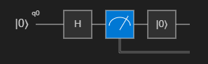
The circuit is displayed in the Q# circuit window. For example, the following circuit corresponds to an operation that puts a qubit in a superposition state and then measures the qubit. The circuit diagram shows one qubit register that's initialized to the $\ket{0}$ state. Then, a Hadamard gate is applied to the qubit, followed by a measurement operation, which is represented by a meter symbol.

View circuit diagrams for operations

To visualize the quantum circuit for a single Q# operation, choose the Circuit code lens above the operation declaration.

View circuit diagrams when you're debugging

When you use the VS Code debugger in a Q# program, you can visualize the quantum circuit based on the current state of the program.

1. Choose the Debug command from the code lens above your entry point operation.

2. In the Run and Debug pane, expand the Quantum Circuit dropdown in the VARIABLES menu to show the circuit while you step through the program.

   

3. Set breakpoints and step through your code to see how the circuit updates as your program runs.

4. The current quantum circuit is shown in the QDK Circuit panel. This circuit diagram represents the current state of the simulator, which is the gates that have been applied up until the current point in your program.

   

Quantum circuits in Jupyter Notebook

In Jupyter Notebook, you can visualize quantum circuits with the qdk.qsharp and qdk.widgets packages. The widgets package provides a widget that renders a quantum circuit diagram as an SVG image.

View circuit diagrams for an entry expression

1. In VS Code, open the View menu and choose Command Palette.

2. Enter and select Create: New Jupyter Notebook.

3. In the first cell of the notebook, run the following code to import the qsharp package.

   from qdk import qsharp
   

4. Create a new cell and enter your Q# code. For example, the following code prepares a Bell State:

   %%qsharp
   
   // Prepare a Bell State.
   operation BellState() : Unit {
       use register = Qubit[2];
       H(register[0]);
       CNOT(register[0], register[1]);
   }
   

5. To display a simple quantum circuit based on the current state of your program, pass an entry point expression to the qsharp.circuit function. For example, the circuit diagram of the preceding code shows two qubit registers that are initialized to the $\ket{0}$ state. Then, a Hadamard gate is applied to the first qubit. Finally, a CNOT gate is applied where the first qubit is the control, represented by a dot, and the second qubit is the target, represented by an X.

   qsharp.circuit("BellState()")
   

   q_0    ── H ──── ● ──
   q_1    ───────── X ──
   

6. To visualize a quantum circuit as an SVG image, use the widgets package. Create a new cell, then run the following code to visualize the circuit that you created in the previous cell.

   from qdk.widgets import Circuit
   
   Circuit(qsharp.circuit("PrepareBellState()"))
   

   

View circuit diagrams for operations with qubits

You can generate circuit diagrams of operations that take qubits, or arrays of qubits, as input. The diagram shows a wire for each input qubit, along with wires for additional qubits that you allocate within the operation. When the operation takes an array of qubits (Qubit[]), the circuit shows the array as a register of 2 qubits.

1. Add a new cell, and then copy and run the following Q# code. This code prepares a cat state.

   %%qsharp
   
   operation PrepareCatState(register : Qubit[]) : Unit {
       H(register[0]);
       ApplyToEach(CNOT(register[0], _), register[1...]);
   }
   

2. Add a new cell and run the following code to visualize the circuit of the PrepareCatState operation.

   Circuit(qsharp.circuit(operation="PrepareCatState"))
   

Conditions that affect circuit diagrams

When you visualize quantum circuits, the following conditions can affect the appearance of your circuit diagrams.

Dynamic circuits

Circuit diagrams are generated by executing the classical logic within a Q# program and keeping track of all allocated and applied gates. Loops and conditionals are supported as long as they deal only with classical values.

However, programs that contain loops and conditional expressions that use qubit measurement results are trickier to represent with a circuit diagram. For example, consider the following expression:

if (M(q) == One) {
   X(q)
}

This expression can't be represented with a straightforward circuit diagram because the gates are conditional on a measurement result. Circuits with gates that depend on measurement results are called dynamic circuits.

You can generate diagrams for dynamic circuits by running the program in the quantum simulator, and tracing the gates as they're applied. This is called trace mode, because the qubits and gates are traced as the simulation is performed.

The downside of traced circuits is that they only capture the measurement outcome and the consequent gate applications for a single simulation. In the above example, if the measurement outcome is Zero, then the X gate isn't in the diagram. If you run the simulation again, then you might get a different circuit.

Target profile

The QIR target profile that you select affects how circuit diagrams are generated. Target profiles are used to specify the capabilities of the target hardware, and the restrictions that are imposed on the quantum program.

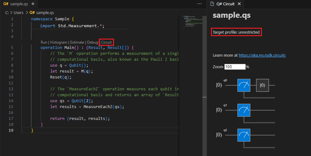
When the target profile is set to Unrestricted, Adaptive RI, or Adaptive RIF, the circuit diagrams show the quantum operations that are invoked in the Q# program. When the target profile is set to Base, the circuit diagrams show the quantum operations that would be run on hardware if the program is submitted to Azure Quantum with this target profile.

Specifically, gate decompositions are applied such that the resulting circuit is compatible with the capabilities of the target hardware. These decompositions are the same ones that get applied during code generation and submission to Azure Quantum.

1. For example, consider the following Q# program that measures a single qubit and an array of qubits.

   import Std.Measurement.*;
   
   operation Main() : (Result, Result[]) {
       // The `M` operation performs a measurement of a single qubit in the
       // computational basis, also known as the Pauli Z basis.
       use q = Qubit();
       let result = M(q);
       Reset(q);
   
       // The `MeasureEachZ` operation measures each qubit in an array in the
       // computational basis and returns an array of `Result` values.
       use qs = Qubit[2];
       let results = MeasureEachZ(qs);
   
       return (result, results);
   }
   

2. When the target profile is set to Unrestricted, Adaptive RI, or Adaptive RIF, the gates in the circuit diagram correspond exactly to the quantum operations that are invoked in the Q# program.

   

3. When the target profile is set to Base, the circuit looks different. Because Base profile targets don't allow qubit reuse after measurement, the measurement is now performed on an entangled qubit instead. The Reset operation isn't a supported gate in the Base profile, so the operation is dropped. The resulting circuit matches what would be run on hardware if this program is submitted to Azure Quantum with this target profile.